conclusions

  1. ML can play an important role in retail challenge today. In the project, naive bayes, SVM, decison tree and other models all shows good example for predicting customer rating, satisfaction, and distinguish the best product in the given scenariom, both customer and business owner will benefit from it

  2. Retailers can gain valuable insights into customer behavior, improve inventory management, optimize pricing strategies, and even for enhancing overall business performance.

  3. The future is bright, but still many problems are waiting to solve on retail industry. For example, the quality of exisitng data, privacy, and model baies, we still have a long way to go.

Regression

1. Overview

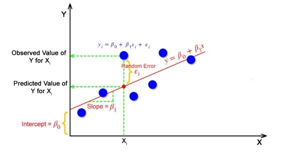
Linear regression is mainly used for builiding the relationship between dependent variable and independent variable. It’s achieved by minimize the sum of square difference between actual and predict values, after optimization round by round, derive the weight and bias for the model.

On other hand, the limitation for linear regression is obvious, as it only works for linear relationship, non-linear relation eg. circle usually has poor performance. Also, it’s sensitive to outliers and easily leads to overfitting.

lr_concept
@Image Source: https://editor.analyticsvidhya.com/uploads/375512.jpg

2. Data Prep

Using the same amazon store sales data as before
sales_raw_data

I did following steps to clean optimize the data.

  1. Keep only numerical value as input feature, for training purpose
  2. Clean and format Numerical data
  3. Outliers removal for some columns

Code Step: https://github.com/BraydenZheng/Product_Recommendation/blob/master/nn/data_prepare.ipynb

Split training and testing data as 80%, 20% portion accordingly.

Taking ‘Actual Price’ as independent variable, ‘discounted Price’ as dependent variable

Cleaned Datalr_dt

3. Code

Model training and evaluation: https://github.com/BraydenZheng/Product_Recommendation/blob/master/nn/regression.ipynb

4. Results

score: 0.57

lr_vs

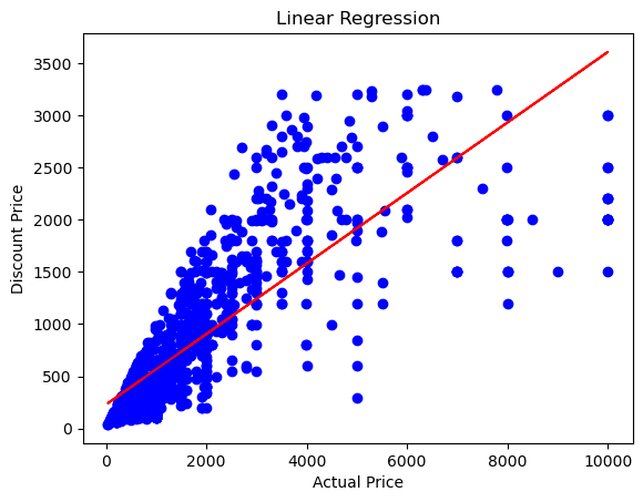
Taking an example for explanation, for the first data row (X=1099), which means this product’s actual_price is 1099, after passing into the trained model (weight=0.33, bias=228), we get result 0.33 * 1099 + 228 = 590. 590 here represent our predited discounted price based on model, and our ground truth discounted price

As it shows on the linear regression graph, data points are concentrated when actual price < 2000, and it becomes quite spread after that, the red line which represents the regression line has a good reflection for the general trend of given dataset, the computed score for model is 0.57, which is not high, but based on visualiztion and data distribtuion, I believe it’s a wonderful training result.

5. Conclusion

Linear regression can be quite useful dealing with simple variable relation, expecially for two variable case ‘dependence’ and ‘independence’ like this one. The major benefit model simplicity and speed can be an effective part when applying to retail store and other big data application.

NN

1. Overview

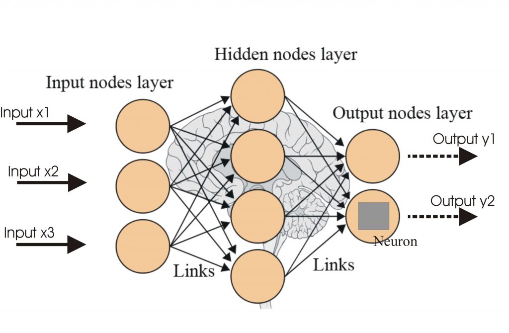
Neural Network is a subfield of machine learning that teach computer to process data in a way that is inspired by human brain. A typical neural network consists of interconnected neurons organized into layers, including an input layer, hidden layers, and an output layer. Each neuron receives and processes input data, passing the results along to the next layer.

Artificial-Intelligence-Neural-Network-Nodes-1024x670
@Image Source: https://raw.githubusercontent.com/BraydenZheng/img/main/uPic/Artificial-Intelligence-Neural-Network-Nodes-1024x670.jpg

2. Data Prep

Using the same amazon store sales data as before

sales_raw_data

I did following steps to clean optimize the data.

  1. Keep only numerical value as input feature, for training purpose
  2. Clean and format Numerical data
  3. Normailze data with standard scaler
  4. Outliers removal for some columns
  5. Discretize the rating column into 2 buckets, and take it as label, in order for classification purpose.

Code Step: https://github.com/BraydenZheng/Product_Recommendation/blob/master/nn/data_prepare.ipynb

Split training and testing data as 80%, 20% portion accordingly.

Lable used here will be rating column, which consist value [0, 1] to stand for good rating / bad rating.

Cleaned Datann_clean

3. Code

Model training and evaluation: https://github.com/BraydenZheng/Product_Recommendation/blob/master/nn/nn.ipynb

4. Results

nn_dis_res

nn_cl

nn_cm

nn_architecture

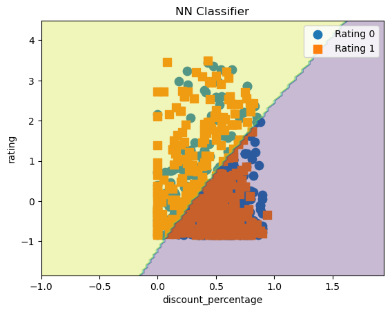
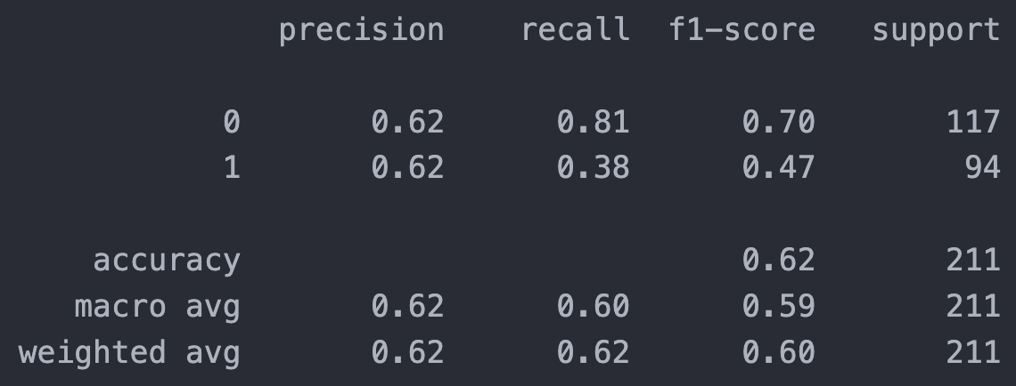
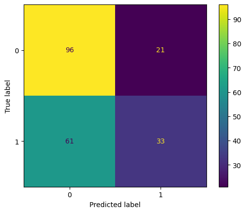
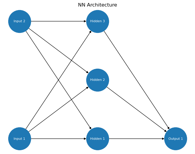
This is basic 3 layers NN network using sigmoid activation function. In general, the library model MLPClassifier has good F-1 score 0.70, providing a balanced measure of both precision and recall. The accuracy is compartively low, which is only 62%.

Regarding to individual label recognizition, Label 0 prediction accuracy are obviously betten than label 1, possibly due to the lack of data and basic level of NN structure.

5. Conclusion

The neural network is a powerful tool for classification tasks. Even a simple NN with few layers and parameters can achieve good performance. However, NNs can also be resource-intensive and time-consuming to train. Striking a balance between resource usage and performance is an important consideration when choosing a NN model, particularly for retail stores with large datasets.

svm

1. Overview:

SVMs are supervised meachine learning techniques massively used in both industry and acamemics for classification, regression purpose.

svm_linear

@Image Source: https://www.analyticsvidhya.com/blog/2021/10/support-vector-machinessvm-a-complete-guide-for-beginners/

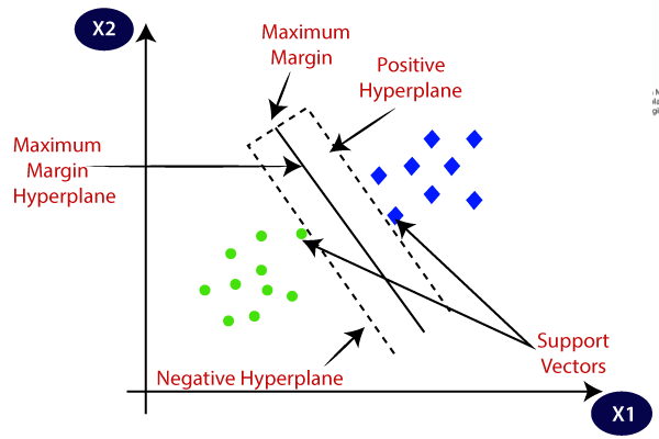
SVMs belong to linear separators because they are used to find a hyperplane to separate the target class in given dataset.

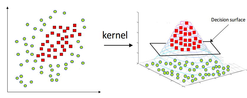
For those dataset can’t be linear separated, svm use kernel trick to cast data into high dimensions and then do the linear separation. The kernel is function that computes the dot product between different points in high dimensional space. This is a crucial step as it doesn’t explicitly calculate the data points in resource expensive high dimensional space, but does it in lower space.

There are two types of most used kernels: Polynomial and RBF kernel:

  1. Polynomial Kernel Function: F(x, y) = (x * y + r)^d. Here x and y refer to input data, r is constant, and d is polynomial degree.

  2. RBF kernel: exp(-γ ||x - y||^2)), here γ = 1/(2σ^2), and σ is a free parameter.

    @Image Source: https://www.hackerearth.com/blog/developers/simple-tutorial-svm-parameter-tuning-python-r/

Let’s consider taking a 2D data point (x, y) and using a polynomial kernel with r = 1 and d = 2 to map the point into a high dimensional space. After expanding the formula:

The new data point pos will be after conversion.

2. Data Prep

Here I use amazon store sales data from kaggle as the raw data, the same raw data used for NaiveBayes.
sales_raw_data
It’s easy to find the original dataset contains lots of text data columns and inconsistent format between numerical columns.

I did following steps to clean optimize the data.

  1. Keep only numerical value as input feature, for navie training purpose
  2. Clean and format Numerical data
  3. Normailze data with standard scaler
  4. Outliers removal for some columns
  5. Discretize the rating column into 3 buckets, and take it as label, the continuous label output didn’t work well for SVM

Code Step: https://github.com/BraydenZheng/Product_Recommendation/blob/master/svm/data_prepare.ipynb

Split training and testing data as 80%, 20% portion accordingly.

The purpose of creating a disjoint split is to ensure that model only testing on unseen data during evaluation, which closely resembles real-world scenarios.

Cleaned Datadata_clean

SVMs can only be used for labbled numerical data, because it relies on mathematical operation likes dot product, and kernel function for optimization also requires numerical input. For those non-numeric data (eg. text input), we need to use encoder, word embedding or other technique to convert them to numeric before passing to SVMs.

3. Code

Model training and evaluation: https://github.com/BraydenZheng/Product_Recommendation/blob/master/svm/svm.ipynb

4. Results

  • Sigmoid Kernel (cost = 1)

    classification_result_sigmoid

    naive_cm_sigmoid

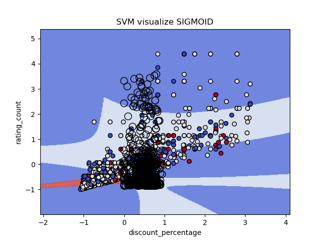
    svm_vis_sigmoid

  • Poly Kernel (cost = 1.2)

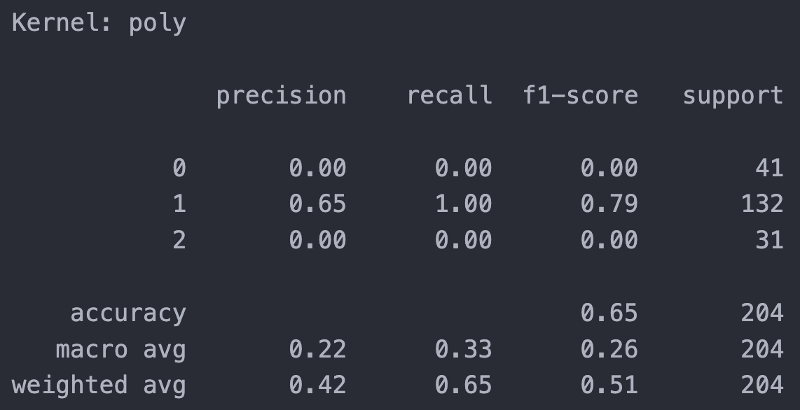
    classification_result_poly

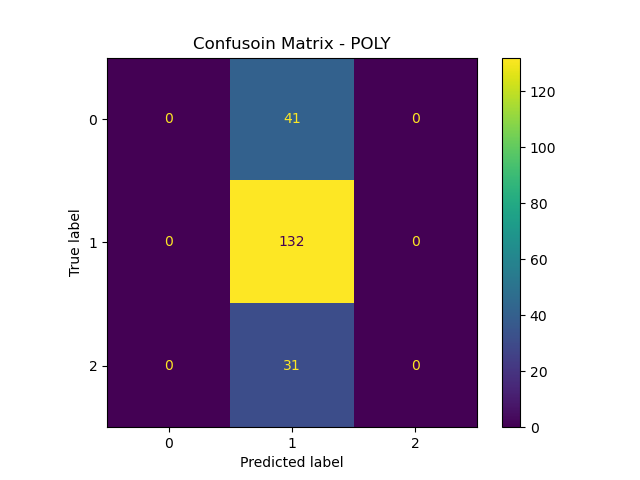
    naive_cm_poly

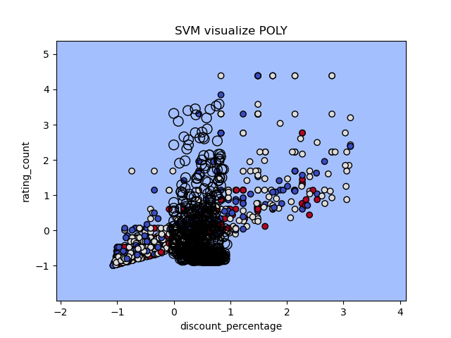
    svm_vis_poly

  • RBF Kernel (cost = 1.5)

classification_result_rbf

naive_cm_rbf

svm_vis_rbf

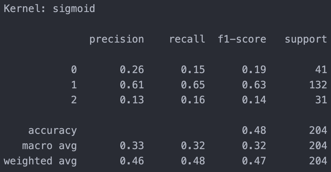
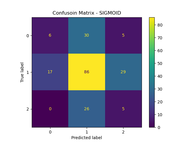
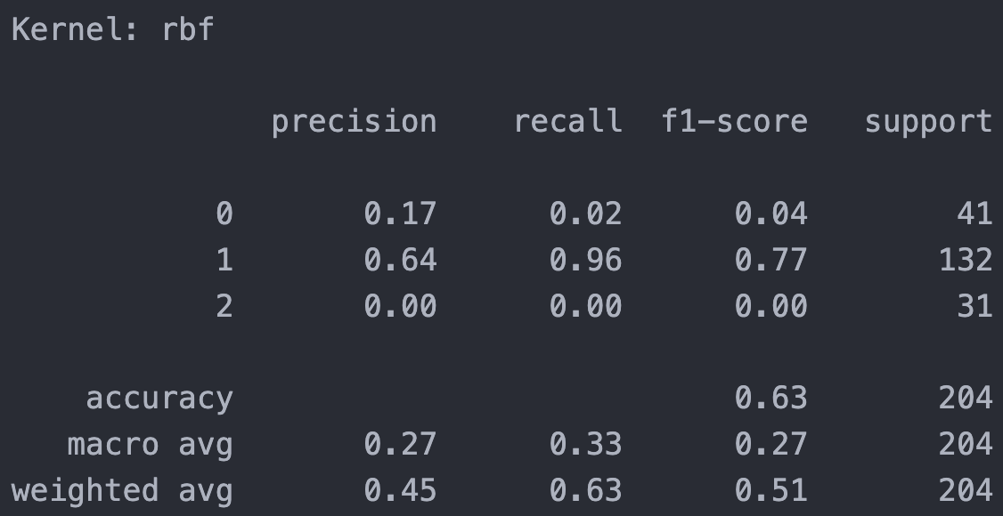
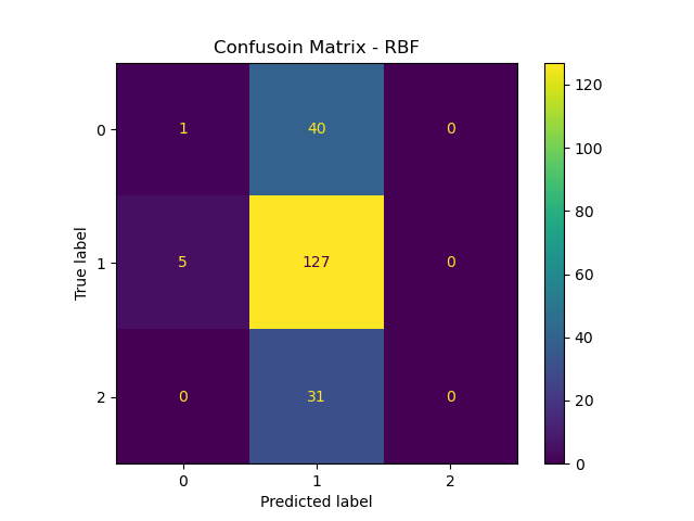
From all kernels result above, the Sigmoid kernel has lowest overall accuracy (48%) , but it performs well in rating class 0 and class 2 compared to other 2 kernels has poor recognization. The performance for RBF and poly are pretty much similar, with better accuracy but failed on class 0 and 2.

For SVM visualization (Re-train with two features), the sigmoid model have good visible boundary for all three class, while other two kernels got boundary gather together.

In general, sigmoid kernel has relative average performance on different class, while RBF and poly kernels has good performance overall and in major class, they didn’t function well in less represented class. For overall rating, I conder ‘sigmoid’ is the best one for this training purpose.

5. Conclusion

  1. The sigmoid model server as general model, it has the ability to take care of every input class even if it’s less represented.
  2. Outliers significantly influences the model performance, when I did the first run without removing outliers, all three functions has super poor result.
  3. While SVM is good way for classification, different kernel has significantly various performance for rating classificaiton purpose, we can change kernels to repspond different needs for the daily business.

DecisonTree

1. Overview

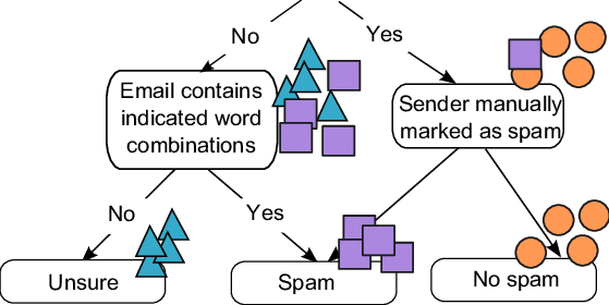
Decison Tree is popular ML algorithm can be applied for both regression and classification problems. The decision tree contains structure called ‘rule’ and ‘node’, where ‘rule’ is the judging condition and leaf is the decison result.

decision_tree

image source: https://www.researchgate.net/figure/A-simple-example-of-a-decision-tree-for-the-classification-of-emails-The-geometric_fig2_265554646

Typical applications includes email spam filter, product classification, and even stock market prediction.

spam_filter

GINI, Entropy, and Information Gain are all used to assist deciding the best rule to split data at each level. They are all useful tools to reduce the impurity of data node, usually we maximize the information gain to make decison tree more effective and use less depth.

Here is an example using GINI and information gain.

Assume we have 10 fruits in total, 7 as apples and 3 as banana.
Before applying any rule, the GINI is: 1 - (P(A)^2 + P(B)^2) = 1 - ((7/10)^2 + (3/10)^2) = 0.42

Then we apply rule 1, for example: weight > 0.2lbs, then we got:
left node: 5 apples and 1 banana
right node: 2 apples and 2 banana

GINI left = 1 - ((5/6)^2 + (1/6)^2) = 0.28
GINI right = 1 - ((1/2)^2 + (1/2)^2) = 0.5

Information gain = 0.42 - (6/10 * 0.28 + 4/10 * 0.5) = 0.05

The information gain 0.05 is a good indicator for how good the split is.

**Why it is generally possible to create an infinite number of trees?**
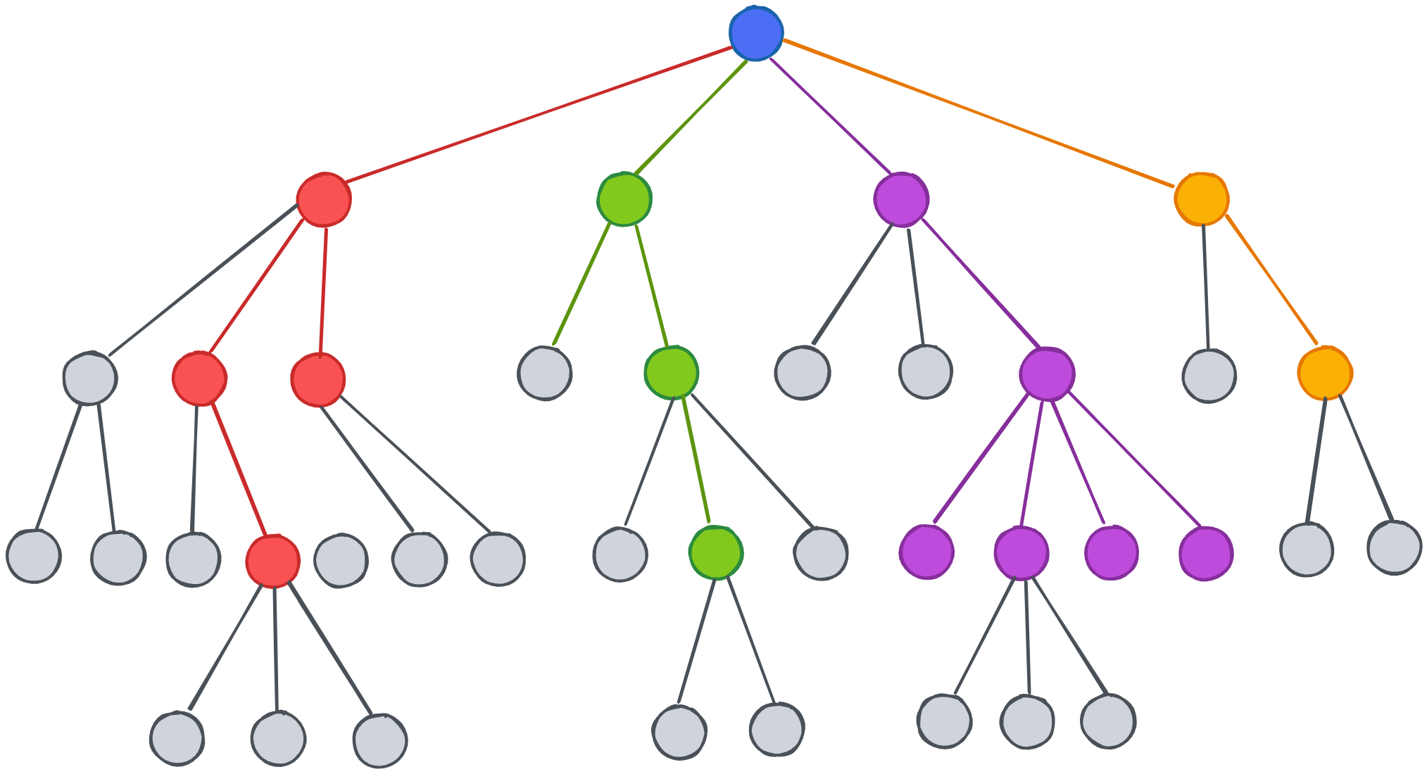
Because there are so many different paramater we can specify for decison tree, such as MaxDepth, GINI or Entropy, also there are many ways for feature representation, each combination above can create a unique tree.

2. Data Prep

Same cleaned sales dataset and testing / training spit method as NaiveBayes model training, however one difference is the data normalization steps are removed, since it’s not useful for DT training and can be confusing when we visualizing the tree.

Code Step: https://github.com/BraydenZheng/Product_Recommendation/blob/master/naivebayes/data_prepare.ipynb

Raw Data
sales_raw_data

Cleaned Data
dt_raw_data

3. Code

Decison Tree training and evaluation:
https://github.com/BraydenZheng/Product_Recommendation/blob/master/decision_tree/decision_tree.ipynb

4. Result

Tree 1

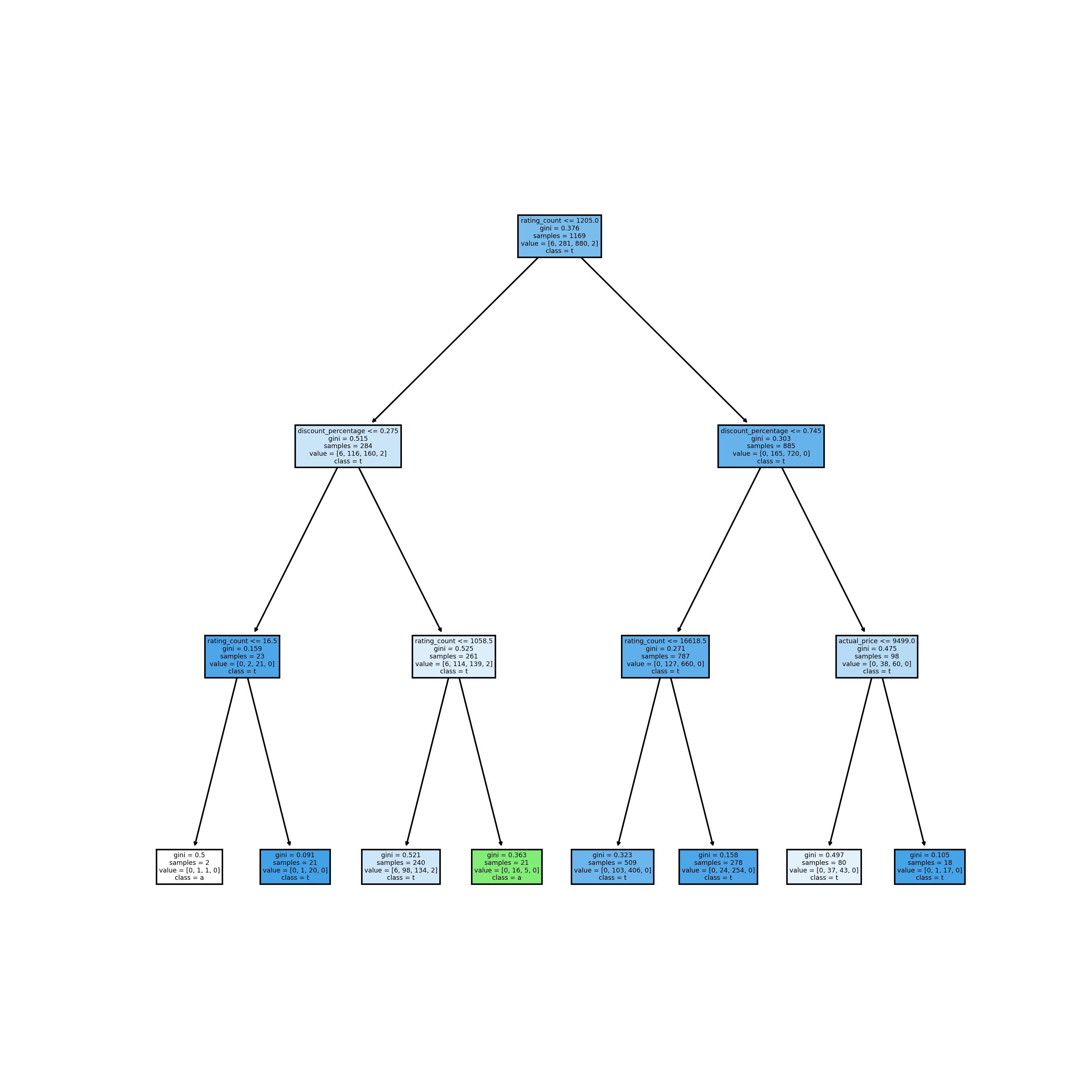
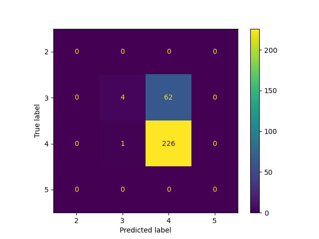
First tree using ‘gini’ as criteria, and max_depth set as 3, achieved the accuracy of 0.78.

tree1
tree1_cm

Tree 2

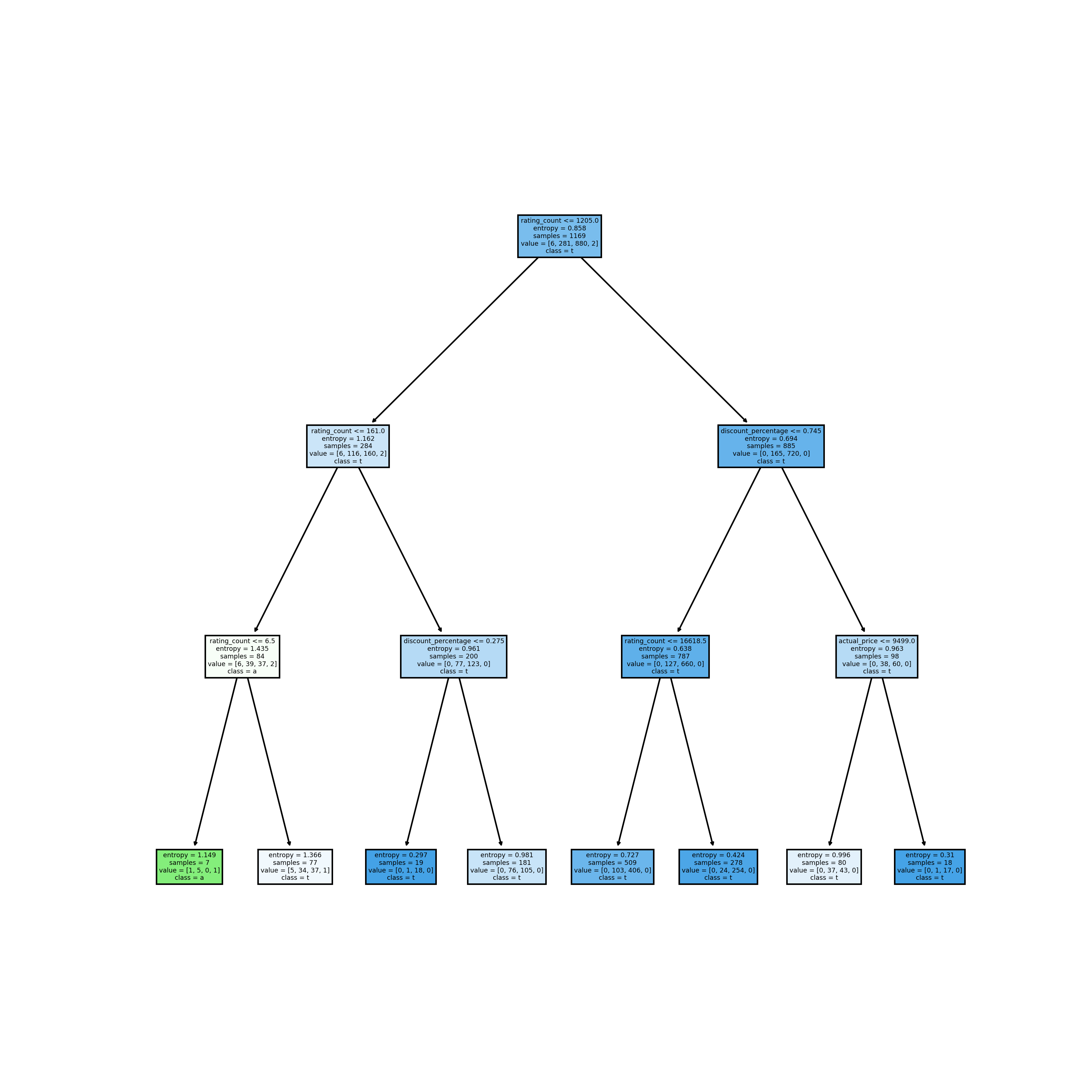
Second tree using ‘entropy’ as criteria, and max_depth set as 3, achieved the accuracy of 0.77.

tree2
tree2_cm

Tree 3

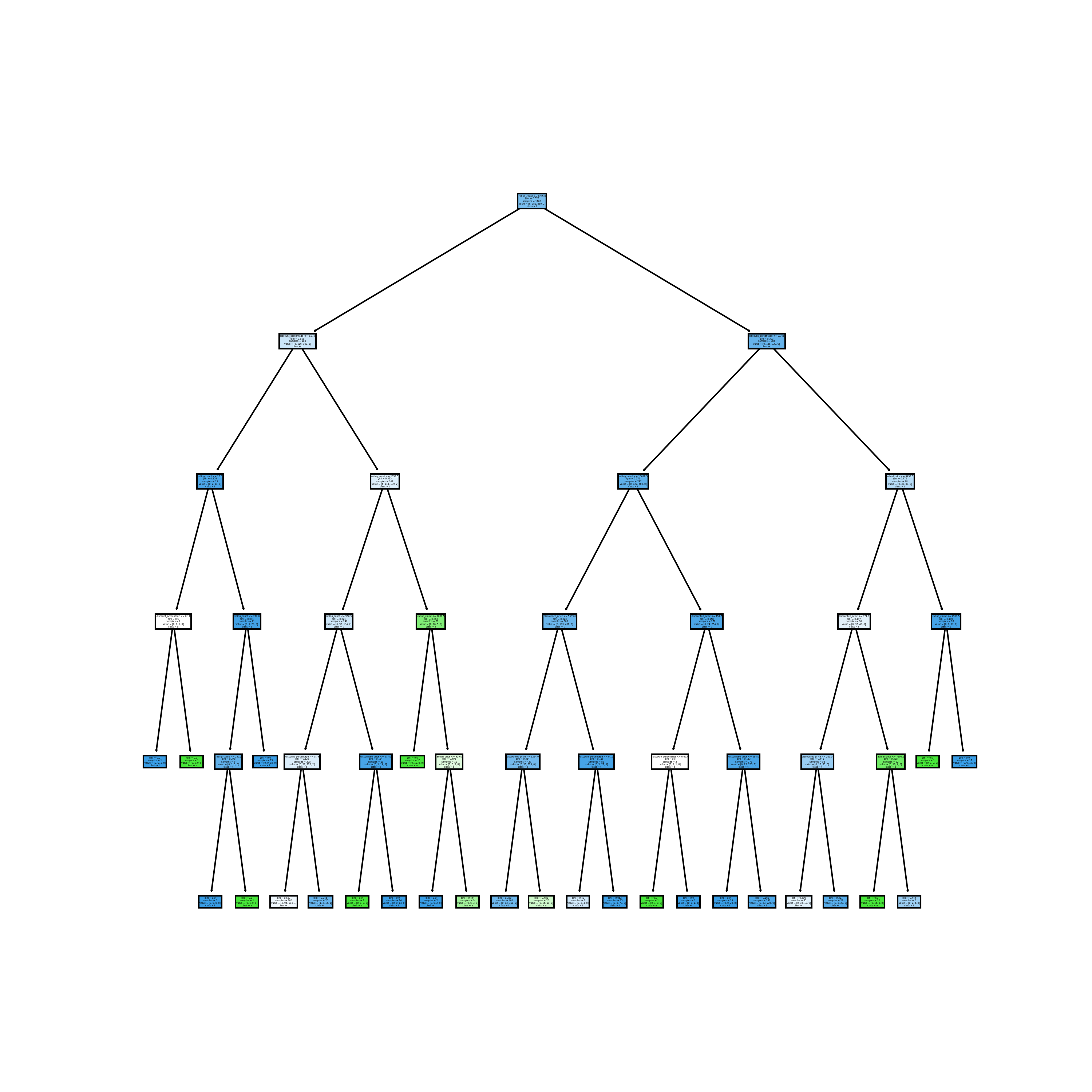
Third tree using ‘gini’ as criteria, and max_depth set as 5, achieved the accuracy of 0.78.

tree3
tree3_cm

From three decison tree results above, we find they all get similar accuracy regardless of parameter setting, which is also close to the one got on NaiveBayes model. Genearlly decison tree has good performance on these numeric data, but training process takes lots of time, especially if we don’t limit the maxiumn depth.

5. Conclusion

Decison tree is a good way to be used for classification, and predicting the rating score in this dataset. We can use this model to predit how customer think about the existing or incoming products, and use these features for future predictions.

NaiveBayes

1. Overview

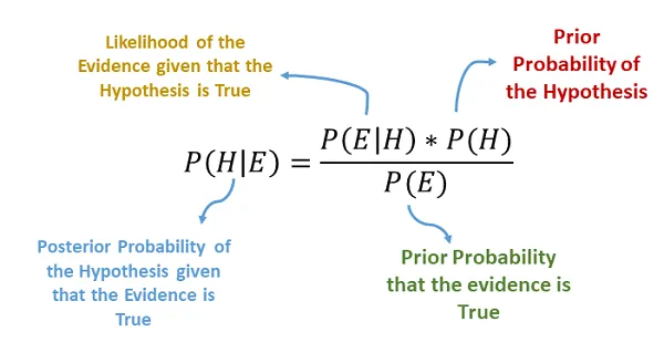
A Naive Bayes classifier is a probabilistic machine learning model used for classification, the most famous implementation is email classification to identify the potential spam.

Multinomial NB algorithm is variant of Naive Bayes, it assumes features are independt, and can be applied to multiple output labels for single model.

Bernoulli is also an naive bayes algorithm mostly used for binary classifcation, and the input features must be binary variable as well (eg. True, False), each feature is considered independent.

Here, we will use Standard Multinomial NB to classify the amazon saling data, and predit an expected rating based on given features.

naivebayes
@Image Source: https://charanhu.medium.com/naive-bayes-algorithm-2a9415e21034

2. Data Prep

Here I use amazon store sales data from kaggle as the raw data.
sales_raw_data
It’s easy to find the original dataset contains lots of text data columns and inconsistent format between numerical columns.

I did following steps to clean optimize the data.

  1. Keep only numerical value as input feature, for navie training purpose
  2. Discretize ‘rating’ column, and take it as label, the continuous label output didn’t work well for NaiveBayes model.
  3. Clean and format Numerical data
  4. Normailze data with min-max scaler

Code Step: https://github.com/BraydenZheng/Product_Recommendation/blob/master/naivebayes/data_prepare.ipynb

Split training and testing data as 80%, 20% portion accordingly

The purpose of creating a disjoint split is to ensure that model only testing on unseen data during evaluation, which closely resembles real-world scenarios.

Cleaned Data
data_clean

3. Code

Model training and evaluation: https://github.com/BraydenZheng/Product_Recommendation/blob/master/naivebayes/naivebayes.ipynb

4. Result

Accuracy: 0.78

naive_cm

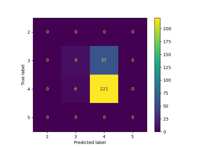
After several rounds of tuning, the model achieve the accuracy 78% on test data. The majority of data has discrete rating as ‘3’ or ‘4’, while model has good performance overall, one weakness of this model is lacking of the ability to predict label rating ‘3’, actullay that’s even not shown on predicted test data.

5. Conclusion

  1. Normalization matters, I got 60% accuracy for data without normalization, the accuracy rise to 78% after applying min-max scaler
  2. Take caution when using MNB for continuous output data. To apply MNB on continuous label, we need to first discretize data label and then feed into the model. However, discretize data sometimes cause the output label too concentrated, which leads to the weakness for model predit on margin data.

ARM

1. Overview

ARM is usually used to find relationships between different elements occured in the dataset. Here, I choose a online retail dataset as the datasource, and brieftly describe the common term used in arm.

Support refers to the frequency of both antecedent and consequent products occur in dataset.

Confidence refer to given the antecedent product, the probability that customer buy the consequent product.

Support-and-Confidence-for-Itemset-A-and-B

@image source: https://www.softwaretestinghelp.com/apriori-algorithm/

Lift is the ratio of support of union antecedent and consequent item to the product of single support of antecent and single support of consequent item.

Rule is an expression of relation between antecedent and consequent items. In the retail dataset, the rule describe the relation that a customer buy certain product based on buy other products.

Apriori algorithm is used to find the association rules given by certain support, confidence, lift and other conditions. The Apriori will start with finding the frequent buying single product in retail example, then based on preset minimum support, confidence, the algorithm only keeps those products satisfy the conditons, and use these products to generate new products sets, it will keep repeating the loop until all rules under conditions found.

apriori
@image source: https://imgbin.com/download/tFwH2qpi

2. Data Prep

Raw data from Kaggle (Online Retail Transaction): https://www.kaggle.com/datasets/mathchi/online-retail-data-set-from-ml-repository
sample_raw_data
Result transaction data:
sample_transaction_data_arm

Generally, I transferred row based transaction data to column based, removed the unused columns, and tested a couple of times for the suitable amount of data, make sure the dataset is not too large to casue out of memory error and not too less which makes graph lack of data point, finally I did some transformation to make it ‘transaction data’ format in R.

Detailed process (Python):
https://github.com/BraydenZheng/Product_Recommendation/blob/master/arm/retail_data_clean.ipynb

3. Code ARM (R)

https://braydenzheng.github.io/arm/skip_render/arm.html

4. Result

Here I set 0.1% support and 0.2 confidence for apriori algorithm argument, with 766911 rules generated, and most of rulse contains one or two items in both antecedent and consequent, product buying relation is low in general, but still many connection between buying behaviour.

**Top 15 rules for lift:**
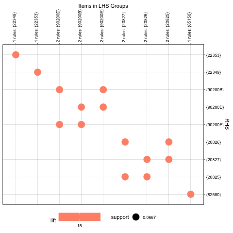
lift_15_group

For the top 15 lift rule, we can see all of these consist of single item, which makes sense for transaction in online retail, single combination (eg. bread + milk) will be most common compared with multiple itemest. Also, the lift value is around 15, we can see the strong connection between antecedent and consequent items there.

**Top 15 rules for confidence:**
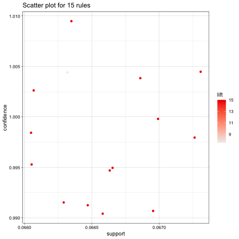
confidence_15
The layout for top 15 confidence rules looks scattered in the plot graph, but actually they are condense with same difference in the value, most high confidence rules has support over 0.06 which is quite high in these dataset with only 200 transcation picked.

**Top 15 rules for support:**
support_15_group
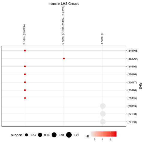
The heighest support went to 0.2 with lift around 6, I do see some grey dot on rightdown corner, with high support but low lift, even it’s single item relation rule, compared with other two graphs above, look like the support is least influcence factor for the strength of association.

5. Conclusion

From the practice and observation above, I see the ‘support’, ‘confidence’, ‘lift’ all play differnet roles in association measurement, depend on the scenario, we may look into ‘support’ for finding the buying association with huge orders base, consider ‘lift’ for the buy together items with strong connection, and finally use these rules to help with the product promption and recommendation.

Clustering

1. Preface

Nowadays, people live in material word with so many choices overwhelming to the daily life, sometimes, finding an item simple as salt would be time-consuming when walking around a big supermarket. Categorize plays a big role to help us limit the search scope, making our searching more easily and quality.
kisspng-cluster-analysis-spectral-clustering-k-means-clust-matrix-code-5ade389a8c0e35.6491918915245129225737

@Source: https://www.cleanpng.com/png-cluster-analysis-spectral-clustering-k-means-clust-1466403/download-png.html

2. Overview

The main object here is clustering / categorizing the best sell amazon book during 2009 ~ 2019, based on year, reviews, prices and other attributes, researchers can find sort of similarity between these books in different styles, customers can have a view of group type and find similar book based on their favourite.
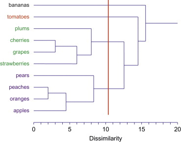
hierarchical
@Source: image from paper Tom Tullis, Bill Albert, in Measuring the User Experience (Second Edition), 2013

Partitional Clustering

Implemented in python, using standard K-means alogrithm for the process, pick a couple of K choices, and use silhouette method and repeat experiment to ensure the clustering quality. Euclidean distance used.

Hierarchical Clustering

Implemented in R, using complete linkage clustering, generating the dendodiagram, and playing around different parameter seting to find a good clustering seperation. Cosine Similarity distance used.

3. Data Prep

For clustering data column, the dataset comes with user rating, number of reviews ,prices, years (publish) as original numerical data type. Besides, ‘Genere_n’ column (filled with value 0/1) will be created based on string type column genere, which indicates whether the book belongs to fiction, will also be used as clustering parameter. Finally, z-score normalization will be applied to some columns.
sample_data
Detail for Data prepartion (Python):
https://github.com/BraydenZheng/Product_Recommendation/blob/master/clustering/data_prepare.ipynb
Link to sample data: book_clustering

4. Code

Code for K-means (Python): https://github.com/BraydenZheng/Product_Recommendation/blob/master/clustering/kmeans.ipynb
Code for Hierarchical Clustering (R): https://braydenzheng.github.io/clustering/skip_render/hierarchical.html

5. Result

5.1 K-Means

At the begining, I tried K = 3 for 5 dimension, althogh 5-D is hard to visualize, I still choose two feature (‘User rating’ and ‘Price’) to visualize the cluster. From picture above, we can see points dense in the center with overlap (500+ points in the graph), but still a clear outline for each cluster.
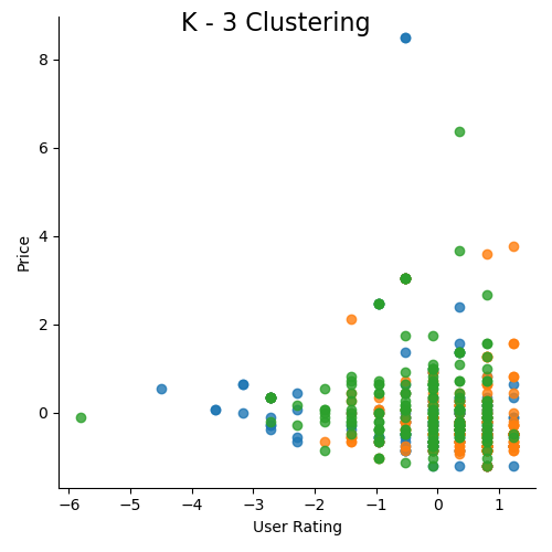
k_3

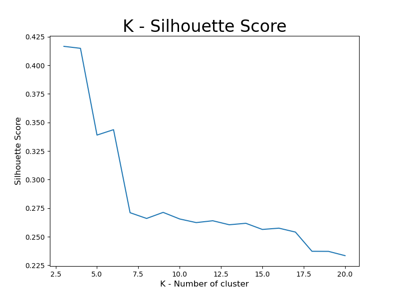
To further discover the best K, I used Silhouette score to try k value range between 3 and 21, and got the graph below.
k_silhouette

Looks like when K equal to around 3, we have best silhouette score, which also shows in the graph with highest score around 0.41. When it goes to 5 or 6, it still have silhouette score around 0.33 while maintaing a good number of clusters, which is a great balance between cluster number and silhouette score.

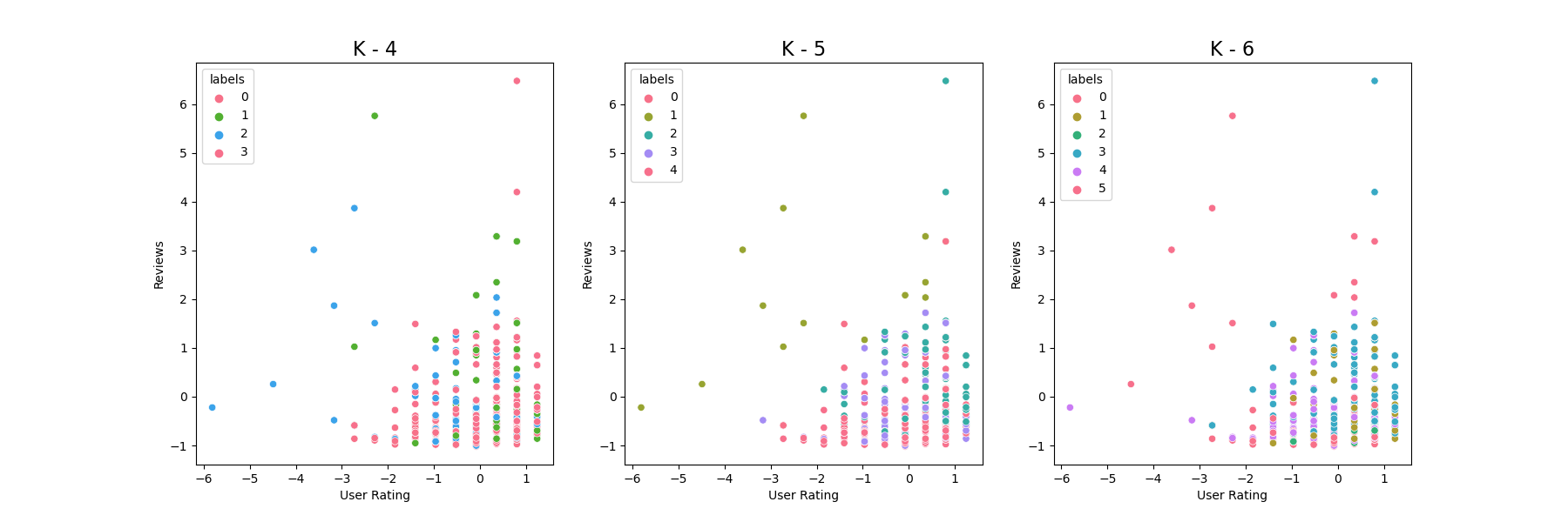
To visualize and decide the best K, I also plot the cluster image for K = 4, 5, 6. (I put 5 features for clustering, in order for plot 2-D, I only choose two features)
k_compare

While it’s hard to determine the best K based on these 2-D graphs, and the three graphs do have dense points gathered in the middle, we still can find the border between each one especially for the outer part, becasue these 3 choices all have good silhouetee score and distribution, I will choose K equal to 6 for a cluster of total 550 books, which will be just on the average so that customer will not feel overwhlemdw with too many categories but also maintains a good variety.

5.2 Hierchical Clustering

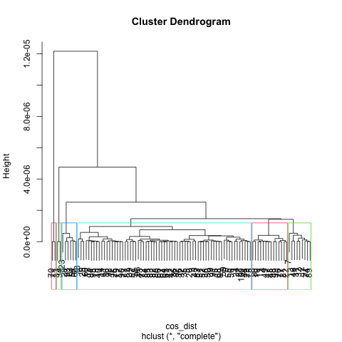
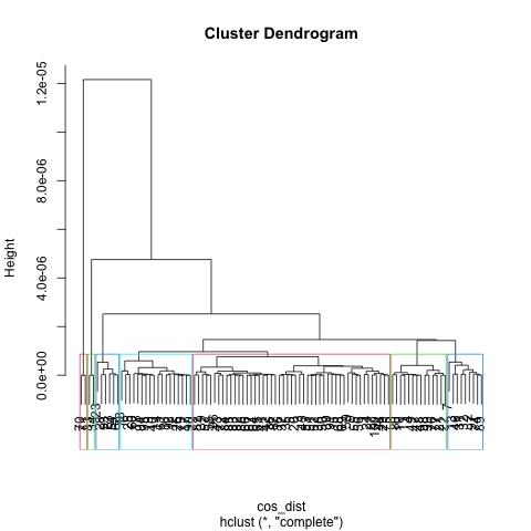
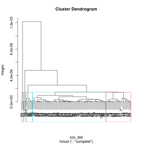
Similar setting is also used for hierarchical clustering, after applying cosine similarity as dist, I tried K as [5, 6, 7] for the clustering, and get graph results below.

K = 5
book_dendrogram_5
K = 6
book_dendrogram_6
K = 7
book_dendrogram_7

From visualization above, one common thing I observe is one cluster took majority of the space (Blue for K == 5, 6 and Red for K == 7). Regards to best K choice, I considered factors that make the tree balanced, having a suitable number of clusters that not too high or too low, also letting each cluster has similar size (keep variance low). K as 7 in this case did best in these valuation factor, which has a good representation of each category also balanced size of the tree.

Compare to K - means, the best K for two algorithms is pretty close (K-means is 6, hclust is 7). For choice in K-means, the silhouette coefficient plays an important role so I choose a small K which makes data points close to each other. For hclust, I consdier more about the tree balanced and its portion ‘big picture’, both of them lead to a similar result at the end.

Conclusions

It’s good practice to apply these two efficient methods for the book clustering, I learned different factors and consideration for find a best K value, that’s also find the number of category for the book recommendation actually. Sometimes, all these values, scores (Silhouette coefficient and tree height), even for distruibtion give us a reference for choosing the K - category, but make a final decison for both K and clustering usually requries extra consideration for business factors or the customer preference.
2.2 download from Kaggle

1
2
3
4
5
6
7
import os
import json
import pandas as pd
import numpy as np
import dataframe_image as dfi
import seaborn as sns
import matplotlib.pyplot as plt

Loading the data downloaded from kaggle

1
df = pd.read_csv('amazon_fine_food/Reviews.csv')
1
df.head(5)

Id ProductId UserId ProfileName HelpfulnessNumerator HelpfulnessDenominator Score Time Summary Text
0 1 B001E4KFG0 A3SGXH7AUHU8GW delmartian 1 1 5 1303862400 Good Quality Dog Food I have bought several of the Vitality canned d...
1 2 B00813GRG4 A1D87F6ZCVE5NK dll pa 0 0 1 1346976000 Not as Advertised Product arrived labeled as Jumbo Salted Peanut...
2 3 B000LQOCH0 ABXLMWJIXXAIN Natalia Corres "Natalia Corres" 1 1 4 1219017600 "Delight" says it all This is a confection that has been around a fe...
3 4 B000UA0QIQ A395BORC6FGVXV Karl 3 3 2 1307923200 Cough Medicine If you are looking for the secret ingredient i...
4 5 B006K2ZZ7K A1UQRSCLF8GW1T Michael D. Bigham "M. Wassir" 0 0 5 1350777600 Great taffy Great taffy at a great price. There was a wid...

Export raw data as image

1
dfi.export(df.head(10), 'img/raw_data.png')

3. Data cleaning and visualize

3.1 Clean irrelevant data column

UserId, profileName, Timestamp is not related to product recommendation, so it’s better to remove them off

1
df = df.drop('UserId', axis = 1)
1
df = df.drop('ProfileName', axis = 1)
1
df = df.drop('Time', axis = 1)
1
df.head(5)

Id ProductId HelpfulnessNumerator HelpfulnessDenominator Score Summary Text
0 1 B001E4KFG0 1 1 5 Good Quality Dog Food I have bought several of the Vitality canned d...
1 2 B00813GRG4 0 0 1 Not as Advertised Product arrived labeled as Jumbo Salted Peanut...
2 3 B000LQOCH0 1 1 4 "Delight" says it all This is a confection that has been around a fe...
3 4 B000UA0QIQ 3 3 2 Cough Medicine If you are looking for the secret ingredient i...
4 5 B006K2ZZ7K 0 0 5 Great taffy Great taffy at a great price. There was a wid...
3.2 Inspect Duplicate Data

1
productId_c = df.iloc[:,1:2]
1
productId_c.head(5)

ProductId count
0 B001E4KFG0 0
1 B00813GRG4 0
2 B000LQOCH0 0
3 B000UA0QIQ 0
4 B006K2ZZ7K 0
1
productId_c.insert(1, 'count',0)

Group by prouduct id to count num of duplicated for each id

1
p_f = productId_c.groupby(['ProductId']).transform('count')
1
p_f.sort_values(by=['count'], ascending=False).head(5)

count frequency
563881 913 913
563615 913 913
563629 913 913
563628 913 913
563627 913 913
1
p_f['frequency'] = 0
1
p_f.head(5)

count frequency
0 1 30408
1 1 30408
2 1 30408
3 1 30408
4 4 17296
1
p_a = p_f.groupby(['count']).count()

Group by count got early to calculate frequency for each duplicate number

1
p_a['frequency'] = p_f.groupby(['count']).transform('count')
1
p_a.iloc[:,0]
count
1      30408
2      24524
3      20547
4      17296
5      15525
       ...  
564     5076
567      567
623      623
632     2528
913      913
Name: frequency, Length: 283, dtype: int64
1
p_a.index
Int64Index([  1,   2,   3,   4,   5,   6,   7,   8,   9,  10,
            ...
            491, 506, 530, 542, 556, 564, 567, 623, 632, 913],
           dtype='int64', name='count', length=283)
1
p_a.head(5)

frequency
count
1 30408
2 24524
3 20547
4 17296
5 15525

Build an image showing the num of duplcated product existed in data set, it’s tremendous

1
2
3
4
5
6
7
8
9
# Horizontal Bar Plot show duplicated count - num of products
plt.bar(p_a.index, p_a.iloc[0])

plt.xlabel("duplicated count")
plt.ylabel("num of products")
plt.title("duplicated products ditribution")
plt.savefig('img/duplicated_product_distribution.png')
# Show Plot
plt.show()

png

3.3 Merge Duplicated Data

The main focus here is merging duplicated data, making each product id unique

For those product contains multiple scores, counting an average probably be a good choice for it. The drawback is some unique fields also need to be removed (‘Text’, ‘Summary’). Since the score plays a determined factor in recommendation, removing is necessary for certain analysis.

1
df_avg = df.iloc[:, 1:5]
1
df_avg

ProductId HelpfulnessNumerator HelpfulnessDenominator Score
0 B001E4KFG0 1 1 5
1 B00813GRG4 0 0 1
2 B000LQOCH0 1 1 4
3 B000UA0QIQ 3 3 2
4 B006K2ZZ7K 0 0 5
... ... ... ... ...
568449 B001EO7N10 0 0 5
568450 B003S1WTCU 0 0 2
568451 B004I613EE 2 2 5
568452 B004I613EE 1 1 5
568453 B001LR2CU2 0 0 5

568454 rows × 4 columns

1
avg = df_avg.groupby(['ProductId']).mean()
1
avg.insert(0, 'ProductId', avg.index)
1
avg.index = range(len(avg.index))

Cleaned Data generated, duplicated value eliminated

1
avg

ProductId HelpfulnessNumerator HelpfulnessDenominator Score
0 0006641040 3.027027 3.378378 4.351351
1 141278509X 1.000000 1.000000 5.000000
2 2734888454 0.500000 0.500000 3.500000
3 2841233731 0.000000 0.000000 5.000000
4 7310172001 0.809249 1.219653 4.751445
... ... ... ... ...
74253 B009UOFTUI 0.000000 0.000000 1.000000
74254 B009UOFU20 0.000000 0.000000 1.000000
74255 B009UUS05I 0.000000 0.000000 5.000000
74256 B009WSNWC4 0.000000 0.000000 5.000000
74257 B009WVB40S 0.000000 0.000000 5.000000

74258 rows × 4 columns

1
avg['HelpfulRatio'] = avg['HelpfulnessNumerator'] / avg['HelpfulnessDenominator']

Replace NAN value with 0

1
avg["HelpfulRatio"] = avg["HelpfulRatio"].replace(np.nan, 0)
1
avg

ProductId HelpfulnessNumerator HelpfulnessDenominator Score HelpfulRatio
0 0006641040 3.027027 3.378378 4.351351 0.896000
1 141278509X 1.000000 1.000000 5.000000 1.000000
2 2734888454 0.500000 0.500000 3.500000 1.000000
3 2841233731 0.000000 0.000000 5.000000 0.000000
4 7310172001 0.809249 1.219653 4.751445 0.663507
... ... ... ... ... ...
74253 B009UOFTUI 0.000000 0.000000 1.000000 0.000000
74254 B009UOFU20 0.000000 0.000000 1.000000 0.000000
74255 B009UUS05I 0.000000 0.000000 5.000000 0.000000
74256 B009WSNWC4 0.000000 0.000000 5.000000 0.000000
74257 B009WVB40S 0.000000 0.000000 5.000000 0.000000

74258 rows × 5 columns

1
dfi.export(avg.head(10), 'img/clean_data.png')
objc[5257]: Class WebSwapCGLLayer is implemented in both /System/Library/Frameworks/WebKit.framework/Versions/A/Frameworks/WebCore.framework/Versions/A/Frameworks/libANGLE-shared.dylib (0x7ffb59f48ec8) and /Applications/Google Chrome.app/Contents/Frameworks/Google Chrome Framework.framework/Versions/109.0.5414.119/Libraries/libGLESv2.dylib (0x111ded880). One of the two will be used. Which one is undefined.
[0206/204727.828076:INFO:headless_shell.cc(223)] 60469 bytes written to file /var/folders/0t/vj81lwzn36xcslx3y2f148t40000gn/T/tmp9j9u523o/temp.png

3.4 Outlier detection

Part of visualization (outlier) code reference from: https://medium.com/swlh/identify-outliers-with-pandas-statsmodels-and-seaborn-2766103bf67c

Method 1: Detect outlier based on Histograms

1
ax = sns.distplot(avg.Score, hist=True, hist_kws={"edgecolor": 'w', "linewidth": 3}, kde_kws={"linewidth": 3})
/var/folders/0t/vj81lwzn36xcslx3y2f148t40000gn/T/ipykernel_3210/869401958.py:1: UserWarning: 

`distplot` is a deprecated function and will be removed in seaborn v0.14.0.

Please adapt your code to use either `displot` (a figure-level function with
similar flexibility) or `histplot` (an axes-level function for histograms).

For a guide to updating your code to use the new functions, please see
https://gist.github.com/mwaskom/de44147ed2974457ad6372750bbe5751

  ax = sns.distplot(avg.Score, hist=True, hist_kws={"edgecolor": 'w', "linewidth": 3}, kde_kws={"linewidth": 3})

png

1
ax.figure.savefig('img/dist_plot.png')

Method 2: Detect outlier based on Distribution

1
ax = sns.boxplot(avg.Score)

png

1
ax.set(title='Review score box plot')
[Text(0.5, 1.0, 'Review score box plot')]
1
ax.figure.savefig('img/box_plot_score.png')

Based on graph results above, score below 2.0 can be possible outlier, however as it’s shown from second graph, the dot is super dense for those “possible outliers”, in this case, no need to remove outlier at this point.

3.5 Other visualization

1
fig = sns.relplot(data = avg, x = 'HelpfulnessDenominator', y = 'HelpfulnessNumerator').set(title='Helpfulness ration among review')

png

1
fig.savefig('img/relation_plot.png')
1
avg.head(5)

ProductId HelpfulnessNumerator HelpfulnessDenominator Score HelpfulRatio
0 0006641040 3.027027 3.378378 4 0.896000
1 141278509X 1.000000 1.000000 5 1.000000
2 2734888454 0.500000 0.500000 3 1.000000
3 2841233731 0.000000 0.000000 5 0.000000
4 7310172001 0.809249 1.219653 4 0.663507
1
fig = sns.residplot(x='HelpfulnessNumerator', y='HelpfulnessDenominator', data=avg, scatter_kws=dict(s=50))

png

1
fig.figure.savefig('img/residual_plot.png')
1
ax = plt.scatter(x= avg.index, y=avg['HelpfulRatio'], color = 'g', s= 0.5)

png

Based on distribution graph, majority of Helpful review ratio concentrate between (0.6, 1)

1
ax.set_xlabel('index')
1
ax.set_ylabel('ratio')
1
ax.title='Review score box plot'
1
ax.figure.savefig('img/Helpful_Ratio_distribution.png')
1
plt.show()

Here comes the graph shows the Helpfulness numberator and Score realtion, generally, most of review get average helpfulness count regardless of score

1
sns.relplot(data = avg, x = 'Score', y = 'HelpfulnessNumerator', color = 'purple')
<seaborn.axisgrid.FacetGrid at 0x7f7b6b9c9960>

png

1
avg_int = avg
1
avg_int['Score'] = avg['Score'].astype(int)

make review score five category, plot distribution of differenct helpfulness indictaors in next 3 graphs

1
sns.catplot(data = avg_int, x = 'Score', y= 'HelpfulnessNumerator', kind = 'bar')
<seaborn.axisgrid.FacetGrid at 0x7f7ad889e200>

png

1
sns.catplot(data = avg_int, x = 'Score', y = 'HelpfulnessDenominator', kind = 'box')
<seaborn.axisgrid.FacetGrid at 0x7f7bbd0bd150>

png

1
sns.catplot(data = avg_int, x = 'Score', y = 'HelpfulRatio', kind = 'violin')
<seaborn.axisgrid.FacetGrid at 0x7f7babee9690>

png

Raw Data VS Clean Data

Raw Data

1
df.head(5)

Id ProductId UserId ProfileName HelpfulnessNumerator HelpfulnessDenominator Score Time Summary Text
0 1 B001E4KFG0 A3SGXH7AUHU8GW delmartian 1 1 5 1303862400 Good Quality Dog Food I have bought several of the Vitality canned d...
1 2 B00813GRG4 A1D87F6ZCVE5NK dll pa 0 0 1 1346976000 Not as Advertised Product arrived labeled as Jumbo Salted Peanut...
2 3 B000LQOCH0 ABXLMWJIXXAIN Natalia Corres "Natalia Corres" 1 1 4 1219017600 "Delight" says it all This is a confection that has been around a fe...
3 4 B000UA0QIQ A395BORC6FGVXV Karl 3 3 2 1307923200 Cough Medicine If you are looking for the secret ingredient i...
4 5 B006K2ZZ7K A1UQRSCLF8GW1T Michael D. Bigham "M. Wassir" 0 0 5 1350777600 Great taffy Great taffy at a great price. There was a wid...

Clean Data (Manily For quantify analysis purpose)

1
avg.head(10)

ProductId HelpfulnessNumerator HelpfulnessDenominator Score HelpfulRatio
0 0006641040 3.027027 3.378378 4 0.896000
1 141278509X 1.000000 1.000000 5 1.000000
2 2734888454 0.500000 0.500000 3 1.000000
3 2841233731 0.000000 0.000000 5 0.000000
4 7310172001 0.809249 1.219653 4 0.663507
5 7310172101 0.809249 1.219653 4 0.663507
6 7800648702 0.000000 0.000000 4 0.000000
7 9376674501 0.000000 0.000000 5 0.000000
8 B00002N8SM 0.473684 0.868421 1 0.545455
9 B00002NCJC 0.000000 0.000000 4 0.000000
1
2
import requests
import pandas as pd

Using the amazon price api from rapidapi.com

1
url = "https://amazon-price1.p.rapidapi.com/search"

Here, I am querying a bottom bracket used for replacing on my bicycle

1
2
3
4
5
6
7
8
9
10
querystring = {"keywords":"bottom bracket","marketplace":"ES"}

headers = {
"X-RapidAPI-Key": "hidden here",
"X-RapidAPI-Host": "amazon-price1.p.rapidapi.com"
}

response = requests.request("GET", url, headers=headers, params=querystring)

print(response.text)

Store the result in panda format

1
df = pd.read_json(response.text)
1
df

ASIN title price listPrice imageUrl detailPageURL rating totalReviews subtitle isPrimeEligible
0 B005L83TF4 SUN RACE BBS15 Bottom Bracket 68/127MM-STEEL E... 13,14 € https://m.media-amazon.com/images/I/316upP-m6I... https://www.amazon.es/dp/B005L83TF4 3.8 33 0
1 B006RM70JY The Bottom Bracket (English Edition) 2,99 € https://m.media-amazon.com/images/I/411tM3tvfN... https://www.amazon.es/dp/B006RM70JY 4.5 2 0
2 B075GQJFL1 Bottom Bracket 0,99 € https://m.media-amazon.com/images/I/71jDB9f3AK... https://www.amazon.es/dp/B075GQJFL1 0
3 B075DW91K2 Bottom Bracket 0,99 € https://m.media-amazon.com/images/I/71Tr4XpGvd... https://www.amazon.es/dp/B075DW91K2 0
4 B09D8S31V7 Bottom Bracket Racket 1,29 € https://m.media-amazon.com/images/I/41qG7oY5Ky... https://www.amazon.es/dp/B09D8S31V7 0
5 B08K2WHFS2 Dandy in the Underworld 1,29 € https://m.media-amazon.com/images/I/51UcKxQdUn... https://www.amazon.es/dp/B08K2WHFS2 0
6 B08K2VYJFK Dandy in the Underworld 1,29 € https://m.media-amazon.com/images/I/51UcKxQdUn... https://www.amazon.es/dp/B08K2VYJFK 0
7 B01J5083XQ Solstice 0,99 € https://m.media-amazon.com/images/I/51avvd1duQ... https://www.amazon.es/dp/B01J5083XQ 0
8 B01J5082CS Solstice 0,99 € https://m.media-amazon.com/images/I/51avvd1duQ... https://www.amazon.es/dp/B01J5082CS 0
9 B09J781T8V Soporte Inferior, Bottom Bracket, Token Ninja ... 74,01 € https://m.media-amazon.com/images/I/312Gc5vg36... https://www.amazon.es/dp/B09J781T8V 5.0 1 0

NN